I have started reading about Deep Learning for over a year now through several articles and research papers that I came across mainly in LinkedIn, Medium and Arxiv.

When I virtually attended the MIT 6.S191 Deep Learning courses during the last few weeks (Here is a link to the course site), I decided to begin to put some structure in my understanding of Neural Networks through this series of articles.

I will go through the first four courses:

1. Introduction to Deep Learning
2. Sequence Modeling with Neural Networks
3. Deep learning for computer vision - Convolutional Neural Networks
4. Deep generative modeling

For each course, I will outline the main concepts and add more details and interpretations from my previous readings and my background in statistics and machine learning.

Starting from the second course, I will also add an application on an open-source dataset for each course.

That said, let’s go!

Introduction to Deep Learning

Context

Traditional machine learning models have always been very powerful to handle structured data and have been widely used by businesses for credit scoring, churn prediction, consumer targeting, and so on.

The success of these models highly depends on the performance of the feature engineering phase: the more we work close to the business to extract relevant knowledge from the structured data, the more powerful the model will be.

When it comes to unstructured data (images, text, voice, videos), hand engineered features are time consuming, brittle and not scalable in practice. That is why Neural Networks become more and more popular thanks to their ability to automatically discover the representations needed for feature detection or classification from raw data. This replaces manual feature engineering and allows a machine to both learn the features and use them to perform a specific task.

Improvements in Hardware (GPUs) and Software (advanced models / research related to AI) also contributed to deepen the learning from data using Neural Networks.

Basic architecture

The fundamental building block of Deep Learning is the Perceptron which is a single neuron in a Neural Network.

Given a finite set of m inputs (e.g. m words or m pixels), we multiply each input by a weight (theta 1 to theta m) then we sum up the weighted combination of inputs, add a bias and finally pass them through a non-linear activation function. That produces the output Yhat.

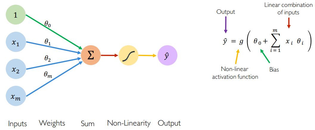
• The bias theta 0 allows to add another dimension to the input space. Thus, the activation function still provide an output in case of an input vector of all zeros. It is somehow the part of the output that is independent of the input.
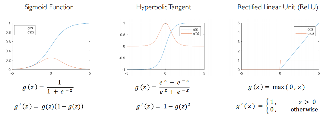
• The purpose of activation functions is to introduce non-linearities into the network. In fact, linear activation functions produce linear decisions no matter the input distribution. Non-linearities allow us to better approximate arbitrarily complex functions. Here some examples of common activation functions:

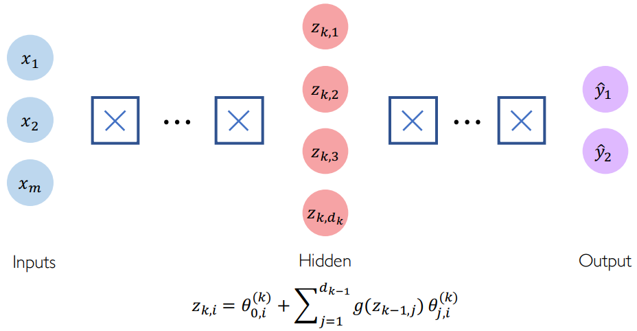
Deep Neural Networks are no more than a stacking of multiple perceptrons (hidden layers) to produce an output.

Now, once we have understood the basic architecture of a deep neural network, let us find out how it can be used for a given task.

Training a Neural Network

Let us say, for a set of X-ray images, we need the model to automatically distinguish those that are related to a sick patient from the others.

For that, machine learning models, like humans, need to learn to differentiate between the two categories of images by observing some images of both sick and healthy individuals. Accordingly, they automatically understand patterns that better describe each category. This is what we call the training phase.

Concretely, a pattern is a weighted combination of some inputs (images, parts of images or other patterns). Hence, the training phase is nothing more than the phase during which we estimate the weights (also called parameters) of the model.

When we talk about estimation, we talk about an objective function we have to optimize. This function shall be constructed to best reflect the performance of the training phase. When it comes to prediction tasks, this objective function is usually called loss function and measures the cost incurred from incorrect predictions. When the model predicts something that is very close to the true output then the loss function is very low, and vice-versa.

In the presence of input data, we calculate an empirical loss (binary cross entropy loss in case of classification and mean squared error loss in case of regression) that measures the total loss over our entire dataset:

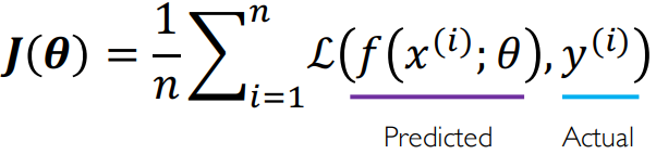
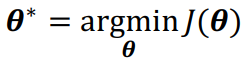
Since the loss is a function of the network weights, our task it to find the set of weights theta that achieve the lowest loss:

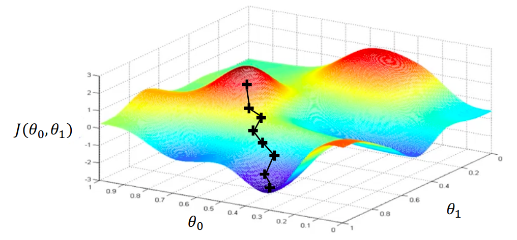
If we only have two weights theta 0 and theta 1, we can plot the following diagram of the loss function. What we want to do is to find the minimum of this loss and consequently the value of the weights where the loss attains its minimum.

To minimize the loss function, we can apply the gradient descent algorithm:

1. First, we randomly pick an initial p-vector of weights (e.g. following a normal distribution).
2. Then, we compute the gradient of the loss function in the initial p-vector.

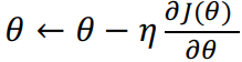
3. The gradient direction indicates the direction to take in order to maximise the loss function. So, we take a small step in the opposite direction of gradient and we update weights’ values accordingly using this update rule:

4. We move continuously until convergence to reach the lowest point of this landscape (local minima).

NB:

• In the update rule, Etha is the learning rate and determines how large is the step we take in the direction of our gradient. Its choice is very important since modern neural network architectures are extremly non-convex. If the learning rate is too low, the model could stuck in a local minimum. If it is too large it could diverge. Adaptive learning rates could be used to adapt the learning rate value for each iteration of the gradient. For more detailed explanation please read this overview of gradient descent optimization algorithms by Sebastian Ruder.

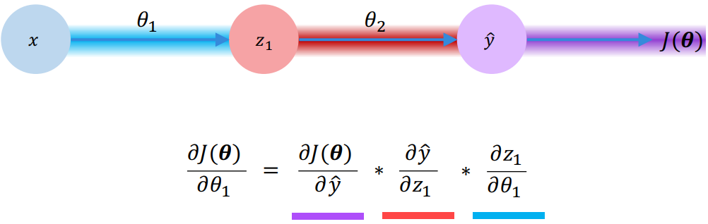
• To compute the gradient of the loss function in respect of a given vector of weights, we use backpropagation. Let us consider the simple neural network above. It contains one hidden layer and one output layer. We want to compute the gradient of the loss function with respect to each parameter, let us say to theta 1. For that, we start by applying the chain rule because J(theta) is only dependent on Yhat. And then, we apply the chain rule one more time to backpropagate the gradient one layer further. We can do this, for the same reason, because z1 (hidden state) is only depend on the input x and theta 1. Thus, the backpropagation consists in repeating this process for every weight in the network using gradients from later layers.

Neural Networks in practice:

• In the presence of a large dataset, the computation of the gradient in respect to each weight can be very expensive (think about the chain rule in backpropagation). For that, we could compute the gradient on a subset of data (mini-batch) and use it as an estimate of the true gradient. This gives a more accurate estimation of the gradient than the stochastic gradient descent (SGD) which randomly takes only one observation and much more faster than calculating the gradient using all data. Using mini-batches for each iteration leads to fast training especially when we use different threads (GPU’s). We can parallelize computing for each iteration: a batch for each weight and gradient is calculated in a seperate thread. Then, calculations are gathered together to complete the iteration.

• Juste like any other “classical” machine learning algorithm, Neural Networks could face the problem of overfitting. Ideally, in machine learning, we want to build models that can learn representations from a training data and still generalize well on unseen test data. Regularization is a technique that constrains our optimization problem to discourage complex models (i.e. to avoid memorizing data). When we talk about regularization, we generally talk about Dropout which is the process of randomly dropping out some proportion of the hidden neurals in each iteration during the training phase (dropout i.e. set associated activations to 0) and/or Early stopping which consists in stopping training before we have a chance to overfit. For that, we calculate the loss in training and test phase relative to the number of training iterations. We stop learning when the loss function in the test phase starts to increase.

Conclusion:

This first article is an introduction to Deep Learning and could be summarized in 3 key points:

1. First, we have learned about the fundamental building block of Deep Learning which is the Perceptron.
2. Then, we have learned about stacking these perceptrons together to compose more complex hierarchical models and we learned how to mathematically optimize these models using backpropagation and gradient descent.
3. Finally, we have seen some practical challenges of training these models in real life and some best practices like adaptive learning, batching and regularization to combat overfitting.

The next article will be about Sequence modeling with Neural Networks. We will learn how to model sequences with a focus on Recurrent Neural Networks (RNNs) and their short-term memory and Long Short Term Memory (LSTM) and their ability to keep track of information throughout many timesteps.

Stay tuned!